
By: Ava Spurr, Chen-Pang Yeang, Patrick Finnigan
September 26, 2023
Introduction:
In this section, we investigate the replication experiments using the galvanometer apparatus to recreate and conduct measurements reminiscent of those conducted at the University of Toronto during the late 19th to early 20th century. As previously outlined, these replication experiments encompass the measurement of electric current using the galvanometer, reaffirming the proportional relationship between deflection and current. We will also address the measurement of low resistance using the bridge method, the determination of the galvanometer resistance, and the calculation of the galvanometer constant.
Our objective is to provide a practical and replicable insight into the methods and measurements that characterized early 20th-century galvanometer experiments. These experiments form the basis of our exploration, aiming to uncover the fundamental principles and techniques that students would have used to make such electrical measurements in this period.
The replication experiments using the galvanometer took place in an office on the third floor of Old Vic, Victoria College, at the University of Toronto. The dates of the replication process took place from January- September of 2023.
This lab will proceed as follows.
Methodology:
The methods used for the setup of the experiments can be divided into different sections, each reflecting progress made in prior lab experiments. Initially, the galvanometer was set up using a breadboard with a series of resistors connected to a battery source, then connected to the galvanometer using a series of alligator clips connected to copper wire.
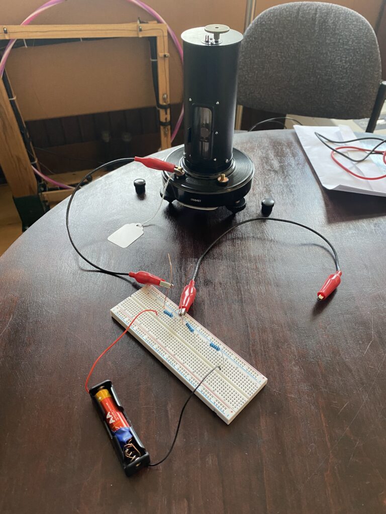
Figure 1: Image of laboratory set-up using the breadboard, alligator clips, AA battery, resistors, and copper wire connected to the galvanometer.
Figure 1 also shows the AA battery fixed with additional materials in the battery box. The battery box that was initially purchased for the lab replications did not match the size of the battery. Thus, to ensure that the battery was sufficiently connected to the rest of the circuit electrical tape and copper wire were fixated to the anode terminal of the battery to connect to the battery box.
The galvanometer’s mirror mechanism was utilized for visualizing and quantifying the deflection of the galvanometer coil, which is directly proportional to the amount of electric charge or current passing through it.
Figure 2: Internal view of the galvanometer showing the mirror at the center attached to the coil.
To facilitate this observation, a laser pointer (one initially meant for pets) served as the light source, directing a focused beam toward the mirror attached to the galvanometer coil. As the coil deflected in response to this light source, the mirror’s angular displacement caused the reflected laser light spot to move accordingly. This movement was then projected onto the adjacent wall (located about 6 feet away, ask Professor Yeang for a more accurate estimate of this distance), allowing for a relatively precise measurement of the deflection angle.

Figure 3: Measuring tape placed on the wall to measure the laser deflection of the galvanometer.
The image above shows how the wall was utilized to measure the deflection angle. During each lab meeting, the galvanometer was set up in a way so that the mirror deflection of the laser would be indicated on the wall, through which a piece of tape would be placed during an incremental increase/decrease of voltage. At first, the increase was made through the addition or removal of resistance on the breadboard attached to the galvanometer, but halfway through our replication process, this was switched to a more consistent power supply. By interpreting this angular displacement and referencing the galvanometer’s calibration, we were able to determine the magnitude of the electrical current.
Please note that each section of the following lab reports using these set-ups will include a more in-depth explanation of each component of the methodology.
Conducting these experiments outside the physics laboratory originally designed for using instruments such as the galvanometer with as little external interference as possible posed several logistical difficulties. Variations in environmental conditions, equipment setup, and resource constraints make the replication process a departure from the controlled and intentionally designed lab setting in which students would have been using this galvanometer.
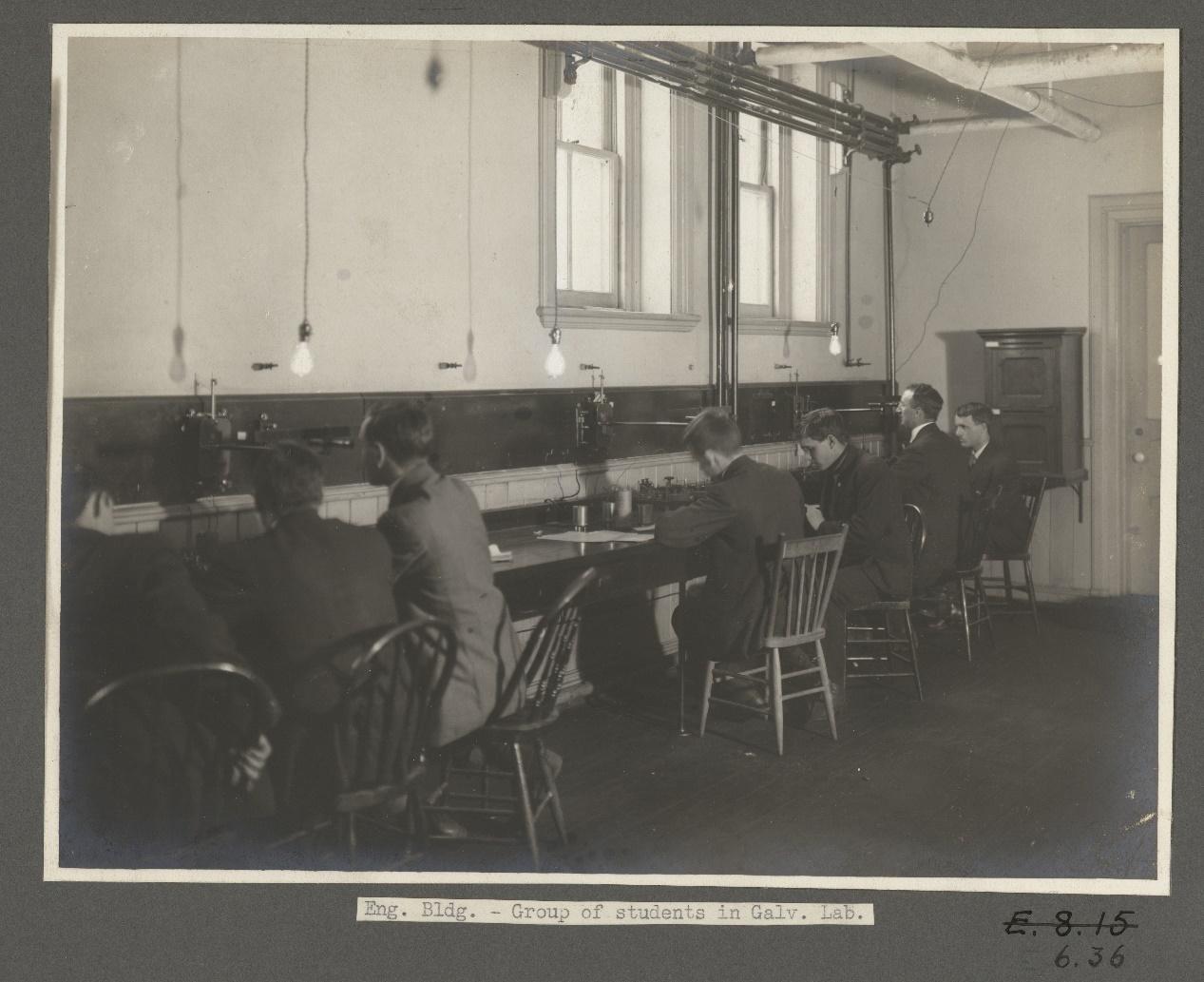
Figure 4: Image of students in physics laboratory designed for use of galvanometer measurements. (UTARMS)
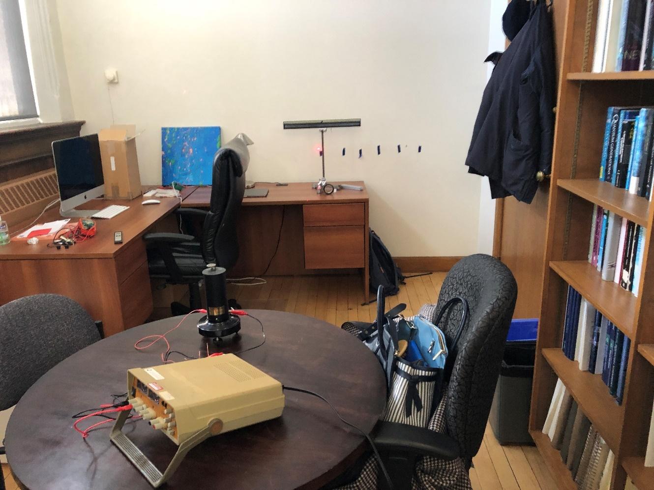
Figure 5: Image from lab setup used in our modern experimental replication.
The age of the galvanometer instrument itself added further difficulties to the replication process. Calibration, a vital process in the setup of the galvanometer, became more challenging due to instrument wear and age-related factors, such as rust and inconsistencies in the range of the mirror deflection. There was also some difficulty encountered in earlier replication lab meetings with getting the galvanometer to be level. This was addressed by using a level and adjusting the screw mechanic on the bottom of the galvanometer to make sure the instrument was level with the light source (pointer laser).
In light of these challenges, our objective remains to provide an academic perspective on the practical difficulties encountered during the replication of early 20th-century galvanometer experiments. Through these difficulties, we aim to gain a comprehensive understanding of the scientific and technical intricacies that characterized the era and its experimental practices. Our replication experiments not only sought to validate historical measurements, but also to shed light on the constraints and adaptability that were inherent in the pursuit of scientific knowledge during that period.

Figure 6: Example of how the Wheatstone Bridge was employed via Thomson’s method, from R.H. Lloyd Fonds.
Observations:
Date: Tuesday, August 9th, 2022
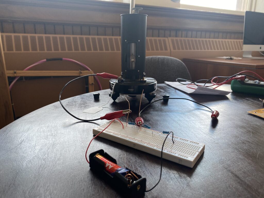
Figure 7: Set up of the Galvanometer with the breadboard.
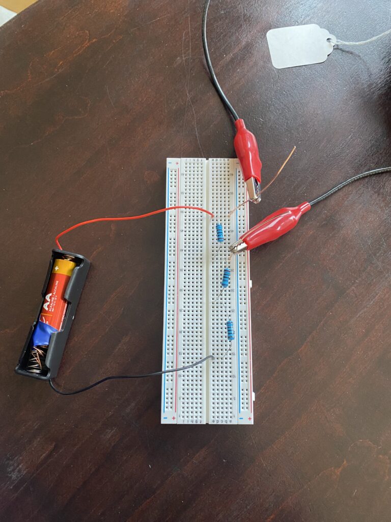
Figure 8: Overview image of the breadboard configuration.
Figure 7 shows the ballistic galvanometer attached to a breadboard containing two resistors in series and one shunt resistor attached in parallel. Figure 8 presents an aerial view of the breadboard being used.
The battery used in the experiment was a 1.5 V AA battery, although the battery box provided was meant for a 3.7 V lithium battery. To address this, copper wire fastened with electrical tape was connected to the negative terminal of the battery (the anode). Three resistors, each with a resistance of 1000 ohms, were employed. Two of these resistors were connected in series on the breadboard, while the third resistor was connected in parallel to the galvanometer on the breadboard using two pieces of copper wire. The experiment revealed that the current caused a deflection in the mirror located inside the galvanometer. However, it was determined that the current was too strong, resulting in an inaccurate reading from the deflection of the mirror. An attempt was made to adjust the current using a variable resistor, but this introduced too much resistance, resulting in no deflection. Based on these results, it was concluded that further experimentation with different resistor values is necessary to obtain variable deflection angles from the provided current.
Set-Up Labs Continued
Date: August 31st, 2022
The purpose of this experiment was to determine a more accurate resistance value for the circuit. During the first experiment trial (refer to section 6.1 experiment data), the deflection was too large, indicating that there was too much current to obtain an accurate reading, as the mirror inside the galvanometer deflected excessively.
| Resistance Value (Ohms) | Deflection Observation |
| 100k | Too little, still noticeable deflection |
| 250k | Too much, no visible deflection |
| 22k | The deflection seems to be good, despite what was initially thought |
| 100k | No deflection |
| 10k | Has a clear deflection, does not go to the extreme. Seems like the best resistance number. |
| 1k | Too small, deflection is too large. |
| 10k | Deflection seems to be good, not too big or small. |
| 22k | Deflection appears even smaller. |
The table above presents resistance values and corresponding deflection observations. These observations were made to determine the most suitable resistance value for the circuit, considering the deflection of the galvanometer. Further experimentation and observations were conducted to refine the resistance choice.
During the lab session on this date, several issues and observations were encountered:
- When connecting the alligator clip to the galvanometer (during the 100k resistor test), the mirror would sometimes not deflect as much. This was initially suspected to be an error within the alligator clip, but the exact cause remained uncertain.
- During a retest of the 100k ohm resistor, it was noticed that the mirror was slowly deflecting over time in one instance, but it did not behave this way when retested.
- Confusing properties were observed with the galvanometer instrument.
- Deflections were not consistently the same even when using the same resistors, and the mirror did not always return to the middle position when the circuit was not connected.
Based on these observations from the experiment date, it was determined that the resistance values for future experiments should fall within the range of 5k to 25k ohms, while maintaining a voltage of 1.5 volts. This range corresponds to a current range of 60 microamps to 300 microamps (A) to ensure that the galvanometer is not saturated. In the subsequent experiment, five resistors ranging from 5k to 25k ohms were used to determine which one was best suited for measuring current with the galvanometer. It was concluded that the issue might be related to the galvanometer itself.
Experiments Continued- Galvanometer Measurements:
Date: January 16th, 2023
Note: Refer to the attached video for a more in-depth look at the experiment.
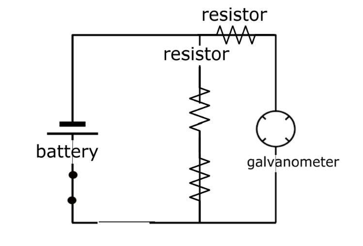
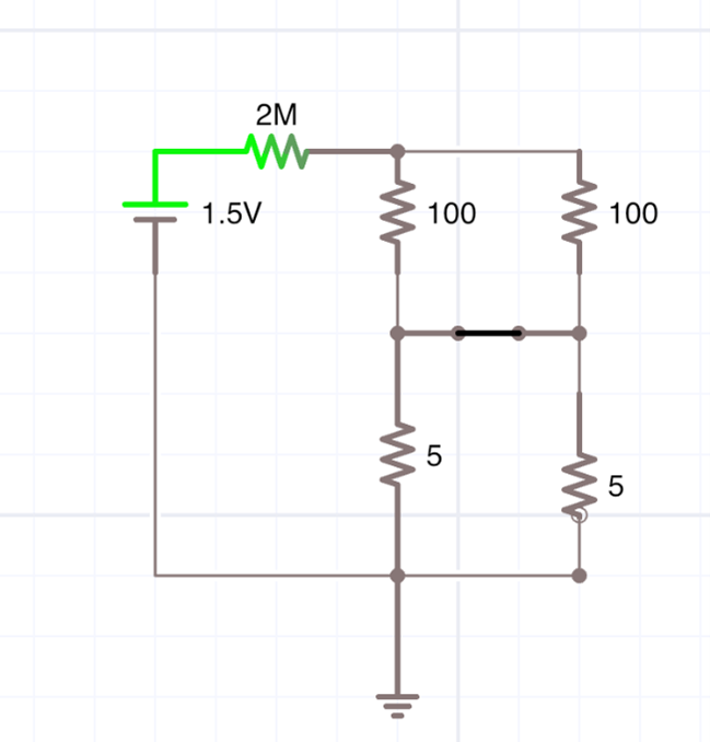
Figure 10: Circuit diagram for galvanometer setup.
In this lab, our team used the galvanometer to measure the deflection from the laser, used by placing tape on the wall at equal increments. This method is something that was also employed for the majority of the following measurements in our lab meetings.
First Deflection Measurement:
Initially, using 10V with the galvanometer did not work. However, this issue was rectified, and the measurement proceeded as planned:
| Voltage (V) | Deflection (Inches) |
| 0 | 10 |
| 2 | 16.5 |
| 4 | 21.6 |
| 6 | 27.0 |
| 8 | 33.0 |
| 10 | 38.9 |
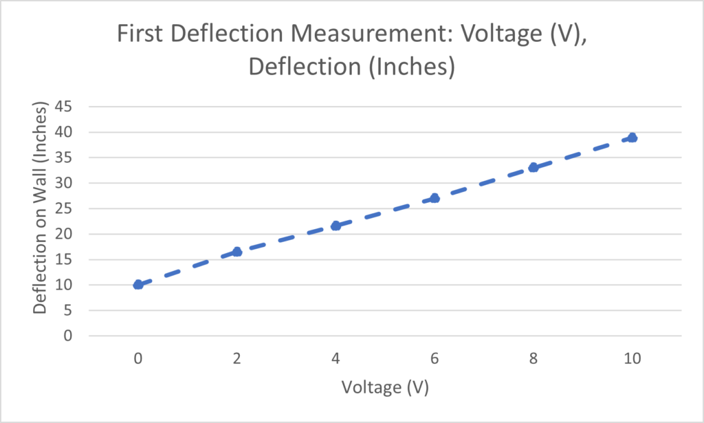
Figure 11: Graph showing the linear relationship between voltage increase, and deflection length on wall.
Note: Sometimes when the voltage was set to zero the laser did not go back to the zero mark.
| Voltage (V) | Deflection (Inches) |
| 0 | 0 |
| 1 | 3.25 |
| 2 | 6.125 |
| 3 | 9.25 |
| 4 | 11.75 |
| 5 | 14.75 |
| 6 | 17.125 |
| 7 | 20 |
| 8 | 23 |
| 9 | 25.5 |
| 10 | 29 |
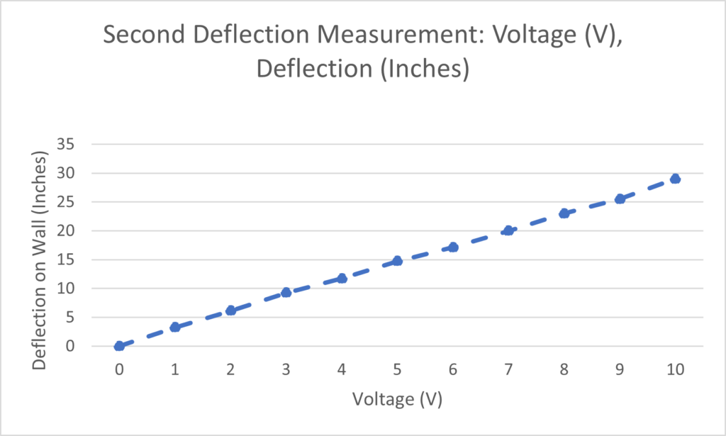
Figure 12: Graph showing the linear relationship between voltage increase, and deflection length on the wall in the second measurement.
Finding the Galvanometer Constant
Date: Monday, February 13th, 2023
In the pursuit of finding the galvanometer constant, it was decided during this lab meeting to exclude the previously used variable resistor while leveraging our understanding of internal resistance. We employed the method of balance to achieve equilibrium between the two arms of the Wheatstone Bridge. The core concept behind the Wheatstone Bridge is to balance two arms against each other. Thomson’s method suggests that if you don’t have a second galvanometer, you can insert a switch to observe current deflection. The aim is to adjust the value of an arm so that when the switch is flipped on or off, the deflection remains the same. This method serves as a means to measure the internal resistance of the galvanometer. A second method, known as Mance’s Method, involves a more extensive series of measurements but is relatively simpler to construct circuit-wise. Mance’s Method: The objective here is to demonstrate that r=ab, where R is the unknown resistance.
One of the techniques used throughout the lab replication experiment is the Equal Deflection Method. This method is commonly employed in electrical measurements to determine an unknown electrical resistance by comparing it to known resistors.
We began with a Wheatstone Bridge circuit, typically comprising four resistors arranged in a diamond shape with a galvanometer connected between two junctions. The galvanometer is employed to detect the balance or equality condition.
The initial step in using this method involves adjusting the values of the known resistors until the galvanometer indicates no current flow, signifying that the bridge is in a balanced state.
Once the bridge is balanced, you can calculate the resistance of the unknown resistor using the fundamental principles of the Wheatstone Bridge: In a Wheatstone Bridge, the ratio of the two known resistors (R1 and R2) is equal to the ratio of the two resistors on the other side of the bridge, with one
of these resistors being the unknown resistor (Rx):
R1R2=RxR3
Where R1 and R2 are the known resistors, Rx is the resistance of the unknown resistor, and R3 is the remaining resistor in the bridge.
From this equation, the value of the unknown resistor (Rx) can be determined by solving for it, allowing for an accurate determination of the unknown resistor’s resistance.
The key insight here is that when the bridge is balanced, the potential difference across the galvanometer is zero, indicating that the ratio of the two known resistors is equal to the ratio of the unknown resistor and the remaining resistor in the bridge. This relationship enables the precise calculation of the value of the unknown resistor. Using a multimeter to measure the current I, we already know the internal resistance, and therefore, there is no need to employ a variable resistor.
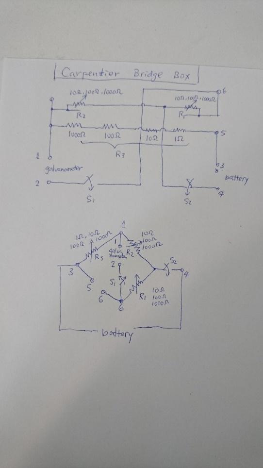
Figure 13: Internal circuit diagram of Carpentier bridge box (left, top), circuit diagram of Carpentier bridge box attached to the battery (left, bottom)
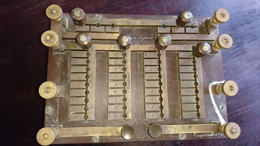
Figure 14: A picture of Carpentier bridge box that was used during this bridge (right).
Finetuning the Experiment
Date: Monday, February 27th, 2023
Following inconclusive results from the previous lab meeting, Pat proposed cleaning the board with a nail file, sandpaper, and a mild acid solution, as there was suspicion that dirt might have been interfering with the measurements.
After the cleaning process, the resistance measurements for 100 ohms and 1000 ohms were found to be accurate. However, the measurement for the 10-ohm resistor showed more fluctuation than desired, hovering around 12 ohms. It was mentioned that such variations are normal for low-resistance measurements, as the meter might have trouble measuring resistance values this low. article geometry.
| Resistance (Ohms) | Trial 1((5 and 3) | Trial 2(1 and 4) | Trial 3(after filing) |
| 10 | 12 | N/A (Doesn’t work) | 11, 10 (switch adjustment needed) |
| 100 | 100 | N/A | 101 |
| 1000 | 1000 | N/A | 1.01k |
The first task was to gain a rough estimate of the galvanometer’s internal resistance through measurement. Then allocate values for a, b, K, and R respectively, just to make sure the values matched/led to a measured internal resistance. This was considered “kind of cheating,” but the purpose was to make sure we had the right values and not waste time endlessly hunting for values.
However, after these tests, the Carpentier bridge box was determined to be too inconsistent to be used for this lab replication experiment.
Measuring the Internal Resistance of Ballistic Galvanometer
Date: May 10th, 2023
The purpose of this lab meeting was to use a new, more modern version of a Wheatstone Bridge (Student Wheatstone Bridge) to measure the internal resistance of the ballistic galvanometer (Figure 15). This new Wheatstone Bridge had no internal connection, and therefore was considered to be a much different design than the previous Wheatstone Bridge that was used during previous experiments.
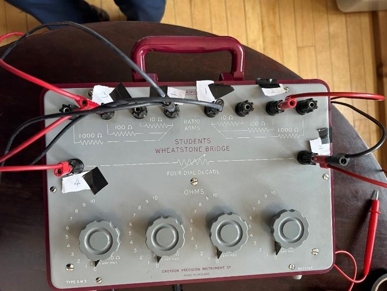
Figure 15: Student Wheatstone Bridge
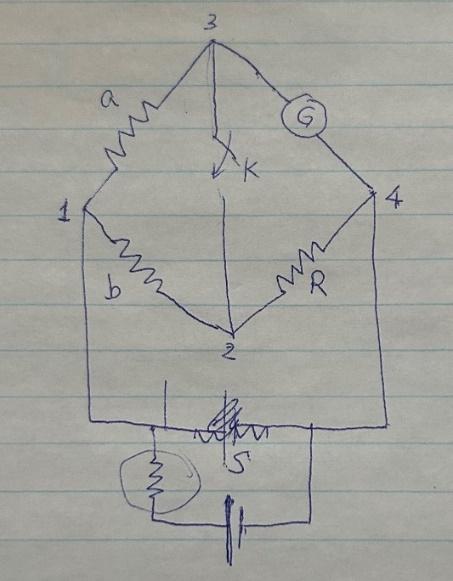
Figure 16: Circuit Diagram of Wheatstone Bridge and Galvanometer (G). Notice in Figure 3 the white labelled pieces of paper indicating the corresponding points on the circuit diagram.
First Test with Switches
- Trying to adjust the value so that when K is on and off it should be the same.
- When the value is adjusted a little bit, notice a deflection.
- When K is not connected it deflects farther, when it is connected it deflects a smaller amount.
| R (Ohms) | Zero-Point | Switch Off (Open) | Switch On (Closed) |
| 5 | 11.5 | 24.5 | 5 ¼ |
| 5 | 11.0 | 25.5 | 5 ¾ |
| 6 | 10.0 | 25.75 | 9 |
| 6 | 11.5 | 24.5 | 5 |
| 7 | 11.0 | 24.3 | 8.5 |
| 8 | 10.5 | No Deflection | No Deflection |
| 8 | 11.0 | 25 | 9 ¼ |
| 9 | 12.0 | 1 | No Deflection |
| 9 | 11.5 | 25.5 | 8 |
| 12 | 9 ¾ | 27 ¼ | 13 ¼ |
| 25 | 9 ¾ | No Deflection | No Deflection |
| 5 | 3 | Very Large Deflection (off the wall) | Very Large Deflection |
Note: Some measurements may not be accurate due to the mirror not being fully released during the experiment. This table is provided for reference and may not be used for drawing conclusions.
Second Test with Switches
(Conducted after the problem was fixed, and the mirror was fully released.)
| R (Ohms) | Zero-Point | Switch Off (Open) | Switch On (Closed) |
| 5 | 1.5 | 7 | 2.5 |
| 6 | 1.5 | 7 | 2.5 |
| 9 | 1.5 | 7.5 | 2.5 |
| 25 | 1.5 | 8 | 3.75 |
| 45 | 2.5 | 9 | 5 |
It was concluded that for the experiment, we might want to do a sensitivity analysis, as the deflection could increase very rapidly for one condition, but decrease very steadily for another condition.
We would then make b = 1000 and a = 100 Expect the balance conditions around 5 ohms, if the window of the balance condition is small, then we would miss it even if we changed the dial to 1. However, if we amplify the window, then we would have a lot more room to work with.
After the Experiment
After the experiment was done with the recorded measurements, we used these values to produce a simulation using iCircuit:
| R | Open Switch | Closed Switch |
| 0.1 | 366 nA | 1.5 nA |
| 3 | 371 | 281 |
| 3.5 | 372 | 309 |
| 4 | 373 | 333 |
| 4.5 | 374 | 355 |
| 5 | 375 | 375 nA |
| 5.5 | 376 | 393 |
| 6 | 377 | 409 |
| 6.5 | 378 | 424 |
| 10 | 384 | 500 |
| 20 | 400 | 600 |
Then, these values were used to produce a graph that showed the results of the simulation:
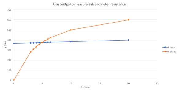
Figure 20: Graph showing ICircuit simulation results from the table in Figure 19.
The ”iCircuit” simulator gives these results for our experimental setup. As you see with the switch open, the current increases gradually. With the switch closed, as in the Thompson experiment – the current increases quite steeply. The curves intersect at the presumed internal G = 5. We found the lead resistance was about 3 – so we assume about 2 more on the dial should add up to 5 to get to a balanced condition.
- Ig did increase slowly with the resistance when the switch was open, however, when it was closed, there was not a rapid increase of Ig (observed much slower)
- Must be why boundary conditions were difficult to produce
As we can see from Figure 20, the current flowing through the galvanometer Ig increases very slowly with the variable resistance R when the switch K in the middle of the bridge is open (blue curve). Meanwhile, Ig increases rapidly with R when K is closed (red curve). Both curves intersect at R = 5Ω.
However, this simulated trend is different from what we observed in this lab meeting. We did see that Ig increases quite slowly with R when K was open, as the blue curve shows. Yet, when K was closed, we did not see a rapid increase of Ig with R. Rather, our observed galvanometer deflection increased quite slowly with R when K was closed, too. This was why we had difficulties producing the balanced condition. And this is puzzling.
Key Takeaways:
- Curve intersection at 5 ohms.
- Different than what was observed in the lab experiment.
Final Experiment
For this lab meeting, our goal was to use the Wheatstone Bridge to find and measure the internal resistance of the galvanometer (RG). In the last meeting, we produced interesting results that were plotted onto a curve, so this meeting, we tried to obtain more measurements to try and find a definitive measurement of the galvanometer’s resistance.
First Deflection Measurement Revisited:
Wheatstone Bridge Data– set at (a=1000Ω, b=100Ω)
Note: The numbers appearing in brackets for the deflection columns are the numbers that the laser was deflected to on the measuring tape. The number of spaces that were deflected are the numbers appearing before this.
| R (Ohm) | Deflection (Switch Closed) | Deflection (Switch Open) |
| 10 | 0.5 (11) | 2.3 (0.8) |
| 20 | 1.1 (11.6) | 2.4 (0.9) |
| 30 | 1.7 (12.2) | 2.6 (1.1) |
| 40 | 2.5 (1) | 2.8 (1.3) |
| 50 | 3 (1.5) | 3 (1.5) |
| 60 | 3.5 (2) | 3.2 (1.7) |
| 70 | 4.1 (2.6) | 3.4 (1.9) |
| 80 | 4.6 (3.1) | 3.5 (2) |
| 90 | 5.2 (3.7) | 3.6 (2.1) |
| 100 | 5.5 (4) | 4 (2.5) |
| 110 | 6 (4.5) | 4.1 (2.6) |
| 120 | 6.5 (5) | 4.3 (2.8) |
| 130 | 6.9 (5.4) | 4.5 (3) |
| 140 | 7.5 (6.0) | 4.7 (3.2) |
| 150 | 8 (6.5) | 4.8 (3.3) |
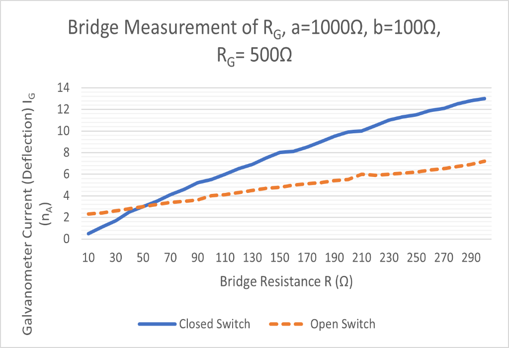
Figure 21: Table and Graph from deflection when a=1000Ω, b=100Ω
From this graph, with a = 1000 ohms and b = 100 ohms, we can see the intersection of the open and closed switch at 50 ohms, implying that the resistance of the galvanometer (RG) is equal to 500 ohms.
- At 50 ohms, both open and closed switch deflections are 3; no change.
Note that this conclusion of RG was initially inconsistent with our initial measurement of the galvanometer’s resistance (8.8 ohms, around 5 ohms). However, it was later found that RG= 500 ohms did make sense after the galvanometer’s resistance was measured again with some adjustments (further explained in the conclusions section).
Second Deflection Measurement:
(a= 100Ω, b=100Ω)
| R (Ohm) | Switch Open | Switch Closed |
| 50 | 1.5 | 7 |
| 100 | 5.5 | 8.5 |
| 200 | 10 | 11.5 |
| 300 | 13 | 14 |
| 400 | 15.5 | 16 |
| 500 | 17.5 | 17.5 |
| 600 | 19 | 19 |
| 700 | 20.5 | 20.5 |
| 800 | 21.5 | 21.5 |
| 900 | 22.5 | 22 |
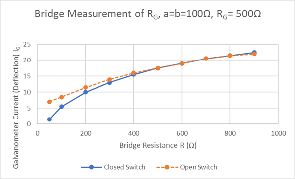
Figure 22: Graph from deflection when a=100Ω, b=100Ω
As we can see from the data points, the curve intersects at 500 ohms, implying that the RG is equal to 500 ohms as well.
The major difference between the data set from a=b=100 ohms and the data set from a=1k ohms and b=100 ohms was that the two curves in the former case entangled together after R=500 ohms, while in the latter case, the closed-switch curve was notably steeper than the open-switch curve. We speculate that the reason for this is that when a=b=100 ohms, the more slowly changing open switch curve intersected with the closed-switch curve at its ”upper” part when the closed-switch curve was no longer that steep.
Conclusions
Both sets of measurements of a = b = 100 Ω, and a = 1000 Ω and b = 100 Ω produced a consistent result of RG≈ 500 Ω. This measurement of the galvanometer’s resistance does make sense, as when the galvanometer was measured again, only this time releasing the mirror of the galvanometer before making the measurement.
The puzzle was then why we obtained a value of RG≈ 5 Ω when we used a multimeter or a multi-function tester to measure across the galvanometer terminals. It was reasoned that this low value was obtained when we locked the galvanometer mirror. But what if we unlocked the mirror and let it wobble while measuring the galvanometer resistance using a multimeter or a multi-function tester? We did just that and found that the value from this measurement was around 500 Ω. That meant that our value from the bridge measurement (RG≈ 500 Ω) was actually correct and consistent with the multimeter reading. Previously, we did not expect that locking and unlocking the galvanometer mirror would make a difference for the galvanometer’s resistance. But it did and changed 100 times! This was new to us. We learned important things about the galvanometer from this experience. This also makes sense as to why the label on the galvanometer has 500 Ω written for the resistance; it was not a mistake and not a result of the ink rubbing off the decimal place, as the value actually is 500 Ω. For reference, refer back to previous Data Plot:

Figure 23: Previous (Bridge 3) Data Plot.